Newton Forward Interpolation is a numerical method used to estimate the values of a function based on a set of known values. This technique is particularly useful when the function is tabulated, and we want to predict values for points that fall within the range of the known data. The method is based on the concept of finite differences and utilizes polynomial interpolation to achieve accurate estimates.
Key Concepts:
Finite Differences: The differences between successive values in a table of data are called finite differences. These differences are used to construct the polynomial interpolation.
Newton's Forward Difference Formula: This method uses forward differences, which involve the data points arranged in increasing order, to compute the interpolated value.
Interpolation Polynomial: The goal is to find a polynomial P(x) that passes through the given data points. Newton’s Forward Interpolation constructs this polynomial based on the first n points.
Numerical methods are essential tools for engineers to solve mathematical problems that are often too complex or impractical to solve analytically. These methods involve approximating solutions using computational techniques, making them invaluable in various fields of engineering.
Common Numerical Methods
Here are some commonly used numerical methods in engineering:
Solution of Algebraic & Transcendental Equations: Techniques to find roots of equations, e.g., Bisection method,Iterative method, Regula falsi method & Newton-Raphson method.
Interpolation: Estimating values between known data points, e.g., Linear interpolation, Lagrange interpolation.
System of Algebraic equations: Gauss Jordan method-Gauss Siedal method.
Numerical Solution of ordinary Differential Equations: The important methods of solving differential equations of first order numerically are as follows, e.g., Taylor's series method, Picard's method, Euler's method, Modified Euler's method of successive approximations and Runge- kutta method.
Optimization: Finding the maximum or minimum of functions, e.g., Gradient descent, Newton's method for optimization.
Finite Element Method (FEM): Numerical technique for solving partial differential equations in engineering and physics.
Comparison of Numerical Methods
Method
Application
Advantages
Disadvantages
Bisection Method
Root finding in continuous functions
Converges reliably, guaranteed to find a root if it exists within the interval
Slow convergence rate, requires initial interval where the function changes sign
Newton-Raphson Method
Root finding, optimization
Faster convergence near the root, suitable for well-behaved functions
Requires derivative, may diverge if initial guess is poor
Trapezoidal Rule
Numerical integration of functions
Simple to implement, generally more accurate than the midpoint rule
Less accurate for functions with high curvature, tends to underestimate the integral
Euler's Method
Numerical solution of ordinary differential equations (ODEs)
Simple and straightforward, easy to implement
Accuracy limited by step size, prone to numerical instability for stiff equations
Finite Element Method (FEM)
Solving partial differential equations (PDEs)
Highly flexible, can handle complex geometries and material properties
These methods are integral to the practice of modern engineering, providing solutions to problems ranging from structural analysis to fluid dynamics and beyond.
Interpolation is a mathematical technique used to estimate values between known data points. It plays a crucial role in various fields such as numerical analysis, computer graphics, and engineering. One popular method for interpolation is the Lagrange interpolation method, named after the French mathematician Joseph-Louis Lagrange.
The Lagrange interpolation method constructs a polynomial that passes through a given set of data points. Suppose you have a set of n+1 data points (x0, y0), (x1, y1), ..., (xn, yn). The Lagrange polynomial, denoted as P(x), is expressed as a linear combination of Lagrange basis polynomials, where each basis polynomial is associated with a specific data point. The general form of the Lagrange polynomial is:
\[P(x) = L_0(x)y_0 + L_1(x)y_1 + \ldots + L_n(x)y_n\]
Here, \(L_i(x)\) is the ith Lagrange basis polynomial, defined as:
\[L_i(x) = \frac{(x-x_0)(x-x_1)\ldots(x-x_{i-1})(x-x_{i+1})\ldots(x-x_n)}{(x_i-x_0)(x_i-x_1)\ldots(x_i-x_{i-1})(x_i-x_{i+1})\ldots(x_i-x_n)}\]
The Lagrange interpolation method provides a flexible and efficient way to approximate values between data points, making it a valuable tool in numerical analysis and scientific computing.
A retaining wall is a structure designed and constructed to hold or retain soil behind it. It is commonly used in landscaping, civil engineering, and construction projects to stabilize slopes, prevent erosion, and create usable spaces on uneven terrain.
Retaining walls are typically built in areas where there is a significant difference in elevation or where there is a need to prevent the movement of soil or rock masses. They are commonly found in residential yards, commercial properties, highways, and agricultural fields.
The primary function of a retaining wall is to resist the lateral pressure exerted by the soil or other materials behind it. This pressure can arise due to factors such as the weight of the soil, water accumulation, or slope inclination. By providing structural support, the retaining wall helps to prevent the soil from sliding or collapsing.
2. where retaining walls are applied in practice ?
Retaining walls are commonly used in various applications where there is a need to hold back soil, earth, or other materials and prevent them from sliding or eroding. Some of the common practical applications of retaining walls include:
Slope Stabilization: Retaining walls are used to stabilize slopes and prevent soil erosion or landslides. They can be constructed on hillsides or steep slopes to provide support and stability to the underlying soil.
Highway and Road Construction: Retaining walls are frequently employed in road and highway construction to create level surfaces and prevent soil from encroaching onto the road. They help in maintaining the integrity of the road and ensure safety for vehicles.
Waterfront Structures: Retaining walls are utilized in waterfront areas to prevent erosion and protect adjacent land from the force of water. They are commonly used along coastlines, riverbanks, and lakeshores to retain the soil and provide stability.
Residential and Commercial Developments: Retaining walls are often incorporated into residential and commercial developments to create usable land on sloping terrain. They are used to create leveled areas for buildings, driveways, parking lots, and landscaped spaces.
Basement and Foundation Support: Retaining walls are employed in building construction to support basements and foundations. They help in preventing the soil around the building from exerting pressure on the structure, ensuring stability and preventing damage.
Landscaping and Garden Design: Retaining walls are used in landscaping and garden design to create terraces, raised flower beds, and seating areas. They add visual interest to the landscape while also providing functional support to the soil and plants.
Railway and Bridge Construction: Retaining walls are utilized in railway and bridge construction to stabilize the embankments and prevent soil movement. They help in maintaining the integrity of the tracks and bridge abutments.
Industrial Applications: Retaining walls find applications in industrial settings such as mining operations, quarries, and storage yards. They provide support to
the surrounding soil and help in managing the storage of materials.
The retaining wall design and construction should be carried out by professionals who consider factors such as soil conditions, water drainage, load requirements, and local regulations to ensure their effectiveness and safety.
3. What are the different types of retaining walls ?
There are several different types of retaining walls, each designed to suit specific conditions and requirements. Here are some common types of retaining walls:
Gravity Retaining Walls: Gravity walls rely on their weight and mass to resist the pressure of the retained soil. They are typically made of concrete or stone and are thicker at the base and gradually taper towards the top. Gravity walls are suitable for lower walls and are cost-effective for retaining moderate heights of soil.
Cantilever Retaining Walls: Cantilever walls are reinforced concrete structures that use a horizontal base called a footing and a vertical wall connected by a horizontal slab or beam. The wall and footing are designed to work together to resist the soil pressure. Cantilever walls are commonly used for medium to high retaining wall heights and can be more economical than gravity walls for larger wall heights.
Sheet Pile Retaining Walls: Sheet pile walls are constructed using interlocking steel, vinyl, or wooden sheets driven into the ground. They are commonly used in waterfront areas and for temporary excavations. Sheet pile walls are effective in soils with limited space and can be easily installed and removed.
Anchored Retaining Walls: Anchored walls use cables or other tensioning devices to provide additional lateral support to the retaining wall. The cables are anchored into the soil or rock behind the wall, creating an anchoring system that resists the soil pressure. Anchored walls are suitable for taller retaining walls or where space is limited.
Gabion Retaining Walls: Gabion walls are constructed by filling wire baskets or cages with rocks or other suitable materials. They are flexible and can accommodate slight settlement without causing structural damage. Gabion walls are often used in landscaping and erosion control applications.
Reinforced Soil Retaining Walls: Reinforced soil walls use layers of soil or granular fill reinforced with geosynthetic materials, such as geotextiles or geogrids. The reinforcing materials add tensile strength to the soil, allowing for taller and more stable walls. These walls are commonly used for highway and bridge construction.
Modular Block Retaining Walls: Modular block walls consist of precast concrete blocks that interlock with each other. They are easy to install and offer flexibility in design. Modular block walls are commonly used in landscaping and residential applications.
Tied-back Retaining Walls: Tied-back walls are similar to anchored walls, but they use horizontal tendons or rods instead of cables for reinforcement. The tendons or rods are anchored into the soil or rock behind the wall, providing additional support.
The selection of the appropriate type of retaining wall depends on factors such as soil conditions, height and load requirements, available space, aesthetics, and project budget. It's important to consult with a qualified engineer or professional to determine the most suitable retaining wall type for a specific application.
The present cantilever retaining wall parts and dimensions.
Three dimension cantilever retaing wall looks like this!!!
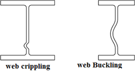
Web buckling refers to the instability or failure of the web of a steel beam under compressive loads. It occurs when the web of the beam is slender and subjected to high compressive forces, causing it to buckle out of its plane.
This phenomenon is more likely to occur in beams with thin webs or when the compressive forces are concentrated over a small area. Web buckling can significantly reduce the load-carrying capacity of a beam.
2. Web Crippling:
Web crippling is the local buckling or failure of the web of a steel beam at points of concentrated load or reaction. It occurs when the web is subjected to high bearing stresses near concentrated loads or reactions, leading to the failure of the web in those specific areas.
This type of failure is common in beams with short spans, high concentrated loads, or when the web is relatively thin. Proper design and detailing are necessary to prevent web crippling.
3. Deflection of Beam:
Deflection of a beam refers to the bending or deformation of the beam under the applied loads. When a beam is subjected to external loads, it undergoes both bending and deflection. Deflection is the displacement of any point on the beam from its original position. The deflection of a beam is influenced by factors such as the magnitude and distribution of the applied loads, the beam's material properties, its length, and the support conditions.
The IS 800 code provides guidelines and limits on deflection to ensure the structural integrity and serviceability of beams.
It's important to note that the specific design considerations, equations, and limitations related to web buckling, web crippling, and deflection of beams can be found in the Indian Standard code IS 800:2007 "General Construction in Steel - Code of Practice."
4. Bending Strength:
Bending strength, also known as flexural strength, is the maximum moment or bending force that a beam can resist before it starts to deform or fail. It is a measure of the beam's ability to resist bending stresses. IS 800 provides specifications and formulas for calculating the bending strength of steel beams based on their cross-sectional properties.
5. Shear Strength:
Shear strength refers to the maximum shear force that a beam can resist before it fails in shear. It is a measure of the beam's resistance to internal forces that cause one part of the beam to slide or shear relative to another part. IS 800 provides guidelines for determining the shear strength of steel beams based on their section properties.
6. What is plastic moment ?
Plastic moment refers to the moment capacity or resistance of a structural member, such as a beam or a column, beyond which the member enters a plastic or fully yielded state. In this state, the material undergoes significant plastic deformation without any increase in load-carrying capacity.
To understand plastic moment, let's consider a simply supported beam with a rectangular cross-section. Initially, when the beam is subjected to increasing loads, it undergoes elastic deformation, meaning it bends but returns to its original shape once the load is removed.
However, as the load increases, the bending moment in the beam also increases. At a certain point, known as the plastic moment, the extreme fibres of the beam's cross-section reach the yield strength of the material. At this moment, the material in the extreme fibres begins to undergo plastic deformation, resulting in permanent changes in shape and size even after the load is removed.
The plastic moment carrying capacity of a section refers to the maximum moment that a structural member or a section can resist before it reaches its fully yielded or plastic state. It represents the ultimate capacity of the section to withstand bending forces without any further increase in load-carrying capacity.
The plastic moment carrying capacity depends on the material properties and the geometry of the section. For a given material, the plastic moment carrying capacity of a section can be determined by considering the plastic stress distribution across the section.
In general, the plastic moment carrying capacity of a section can be calculated using the following formula:
Mp = Zp * fy
where:
Mp is the plastic moment carrying capacity of the section,
Zp is the plastic section modulus, which represents the distribution of material away from the neutral axis, and
fy is the yield strength of the material.
The plastic section modulus, Zp, is calculated based on the shape and dimensions of the section. It takes into account the location of the extreme fibres and their distance from the neutral axis of the section.